Next: Evaluating results - Graphical Up: Dynamical Susceptibility and Excitations Previous: DMD - formalism Contents Index
Physical observables are related to operators such as the magnetic moment components or the scattering operators. We now
introduce a series
of observables
![]() (
(
![]() )
for each subsystem
)
for each subsystem
![]() and define a corresponding correlation function and
dynamical susceptibility. The correlation function we denote as
and define a corresponding correlation function and
dynamical susceptibility. The correlation function we denote as
![]()
Note that the observables
![]() may have some
may have some ![]() dependence (for example if we
consider the Fourier transform of a magnetisation density of
a magnetic ion in a crystal [49]). We
omit this
dependence (for example if we
consider the Fourier transform of a magnetisation density of
a magnetic ion in a crystal [49]). We
omit this ![]() dependence to make notation easier but will come back to it when considering
the calculation of the neutron scattering cross section.
dependence to make notation easier but will come back to it when considering
the calculation of the neutron scattering cross section.
Using the fluctuation-dissipation theorem
![]() can be related to a dynamical susceptibility
can be related to a dynamical susceptibility ![]() :
:
However, in contrast to the dynamical susceptibility
![]() , based
on the operators
, based
on the operators
![]() ,
the susceptibility
,
the susceptibility
![]() cannot be obtained from solving the MF-RPA equation (226).
The reason is that the derivation of (226)
makes use of the dynamical evolution of the operators
cannot be obtained from solving the MF-RPA equation (226).
The reason is that the derivation of (226)
makes use of the dynamical evolution of the operators
![]() and not of the observables
and not of the observables
![]() .
.
Nonetheless, general properties of dynamical susceptibilities may be used
to get a relation between
![]() and
and
![]() .
In general a dynamical susceptibility
.
In general a dynamical susceptibility
![]() describes the response of
a physical observable
describes the response of
a physical observable
![]() to a perturbation of the system described by
an operator
to a perturbation of the system described by
an operator ![]() .
In the case of the dynamical susceptibility corresponding to the observables
.
In the case of the dynamical susceptibility corresponding to the observables
![]() we therefore have to
set
we therefore have to
set
![]() with the definitions
with the definitions
 |
(228) | ||
 |
(229) |
From linear response theory it can be shown [1, page 143], that the dynamical
susceptibilities have poles at the excitation energies of the system: In equation (216)
the denominator, the eigenstates and the difference in thermal population are the same for any susceptibility.
The energy eigenstates
![]() of the system will be a linear combination of
direct products involving
single ion states.
Therefore, the numerator in equation (216) will
be a (usually not known) linear combination of products of the form
of the system will be a linear combination of
direct products involving
single ion states.
Therefore, the numerator in equation (216) will
be a (usually not known) linear combination of products of the form
![]() and
and
![]() for
for
![]() and
and
![]() , respectively.
, respectively.
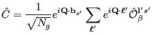
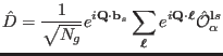
These terms can be related by a similar procedure to that outlined in equations (230) ff. We define the matrices,
similar to the
![]() of equation (230), however, omitting the
thermal population factors and expectation values. These matrices
can be diagonalised using the
unitary transformations
of equation (230), however, omitting the
thermal population factors and expectation values. These matrices
can be diagonalised using the
unitary transformations
![]() (
(
![]() )
and
)
and
![]() (
(
![]() ), respectively.
), respectively.
Again, all eigenvalues are zero except for
![]() and
and ![]() , respectively.
, respectively.
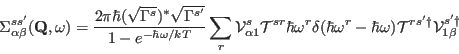
In [35] these transformations are used to derive the following expression for the dynamical susceptibility
Equation (247) shows how knowledge of the dynamical susceptibility calculated
on the basis of the interaction operators between subsystems (
![]() )
may be used to obtain the dynamical susceptibility for any set of observables
)
may be used to obtain the dynamical susceptibility for any set of observables
![]() of
the system.
of
the system.
The standard procedure to avoid divergences is to substitute ![]() with
with
![]() and
take the limit for
and
take the limit for
![]() . Using Dirac's formula
. Using Dirac's formula
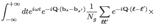
the absorptive part of the dynamical susceptibility (240) becomes
and the correlation function
![]() can be evaluated by applying the
fluctuation dissipation theorem (239):
can be evaluated by applying the
fluctuation dissipation theorem (239):
To keep notation simple, the ![]() dependence of the eigenvectors
dependence of the eigenvectors
![]() and the energies
and the energies ![]() has been omitted.
If the observable
has been omitted.
If the observable
![]() depends explicitly on
depends explicitly on ![]() , then also
, then also
![]() and thus
and thus
![]() will depend on
will depend on ![]() .
This very fundamental result will be applied to the neutron scattering cross section
in section M.
.
This very fundamental result will be applied to the neutron scattering cross section
in section M.
The elastic contribution to equations (249) and
(250) has to be evaluated taking into account
a small but finite value for the energy shift ![]() introduced
in the discussion of equation (227). It turns
out, that
introduced
in the discussion of equation (227). It turns
out, that ![]() and
and ![]() and thus also
the dynamical matrix
and thus also
the dynamical matrix ![]() and its eigenvalues
are proportional to
and its eigenvalues
are proportional to ![]() . Making use of the normalisation
for the eigenvectors
. Making use of the normalisation
for the eigenvectors
![]() we find that the dynamical susceptibility (249)
is proportional to
we find that the dynamical susceptibility (249)
is proportional to ![]() and thus zero in the limit of
and thus zero in the limit of
![]() . However, in the correlation function
(250) the denominator is proportional to
. However, in the correlation function
(250) the denominator is proportional to
![]() leading to a finite result for the quasielastic response.
leading to a finite result for the quasielastic response.