Theory for program bfk - Inelastic neutron-scattering from RE ions in a crystal field including damping effects due to the exchange interaction with conduction electrons

This is an extension of the theory published by Klaus W. Becker, Peter Fulde and Joachim Keller in Z. Physik B 28,9-18, 1977 [4] "Line width of crystal-field excitations in metallic rare-earth systems" and an introduction to the computer program for the calculation of the neutron scattering cross section. The computer program bfk is written by J. Keller, University of Regensburg.

Here we present a brief outline of the theoretical concepts to calculate the dynamical susceptibility of the Re ions and the scattering cross section.

The neutron-scattering cross section is related to the dynamic susceptibility of the RE ions

$$\chi_{\alpha\beta}(t)={i\over \hbar} \Theta(t)\langle [J^\dagger_\alpha(t), J_\beta(0)]\rangle$$

whose Fourier-Laplace transform

$$\chi_{\alpha,\beta}(z)=\int_{-\infty}^{+\infty} dt e^{izt}\chi_{\alpha\beta}(t), \quad z=\omega +i\delta$$

determines the inelastic neutron scattering crossection (Stephen W. Lovesey; "Theory of neutron scattering from condensed matter" Vol 2, equ. 11,144).

$${d^2\sigma \over d\Omega d E'}= {k' \over k}({r_0\over 2}g_J... ...hi{''}_{\alpha,\beta}(\omega)\over 1-e^{-\beta \hbar \omega}}$$

Here $k$ and $k'$ denote the wave number of the neutron before and after the scattering. $\vec Q = \vec k - \vec k'$ is the scattering wave vector, $\tilde Q = \vec Q/\vert\vec Q\vert$. $r_0= -0.54 \cdot 10^{-12}$ cm is the basic scattering length, $g_J$ is the Landé factor, $F(Q)$ the atomic form factor of the rare earth ion.

Formal evaluation of the dynamic and static susceptiblity.

The dynamic spin-susceptibilities are correlation functions of the form

$$\chi_{i,k}(t)=i \Theta(t) \langle [A_i^\dagger(t),A_k(0)]\rangle$$

where $A(t)$ is a Heisenberg operator

$$A(t)= \exp(iHt)A\exp(-iHt)$$

Introducing a Liouville operator (acting on operators of dynamical variables) by ${\cal L}A = [H,A]$ the Heisenberg operator can also be written formally as

$$A(t)= \exp(i{\cal L}t) A$$

With help of this definition the dynamical susceptibility $\chi_{i,k}$ of two variables $A_i, A_k$ can be written as

$$\chi_{i,k}(t)=i \Theta(t) \langle [A_i^\dagger(t),A_k(0)]\rangle$$

and their Laplace transform

$$\chi_{i,k}(z)=i\int_0^\infty dt e^{izt} \langle [A_i^\dagger(t),A_k(0)]\rangle$$

With help of the Liouvillian these quantities can be written as

$$\chi_{i,k}(t)=i \Theta(t) \langle [A_i^\dagger,A_k\exp^{-i{\cal L}t}\rangle$$

and their Laplace transform

$$\chi_{i,k}(z)= -\langle [A_i^\dagger,{1\over {z-\cal L}}A_k(0)]\rangle$$

The static isothermal susceptibilities can also formally be calculated with help of the Liouvillian.

$$\chi_{i,k}(0) = \int_0^\beta d \lambda \langle e^{\lambda H}... ... \lambda \langle (e^{\lambda {\cal L}} A_i^\dagger) A_k\rangle$$

The static susceptibilities are used to define a scalar product between the dynamical variables:

$$(A_i \vert A_k) = {1\over \beta }\int_0^\beta d\lambda \lang... ...da{\cal L}}A_i^\dagger)A_k\rangle ={1\over \beta} \chi_{ik}(0)$$

It fulfills the axioms of a scalar product and furthermore it has the important property

$$({\cal L}A_i\vert A_k)=(A_i\vert {\cal L}A_k)={1\over \beta}\langle [A_i^\dagger,A_k]\rangle$$

With help of this relation the dynamical susceptibility can be expressed as

$$\chi_{i,k}(z)= -\beta (A_i\vert {{\cal L}\over {z-\cal L}} A_k)$$

and finally as

$$\chi_{ik}(z)=\chi_{ik}(0)-z\beta (A_i\vert {1\over {z-\cal L}}A_k)$$

The second term is the so-called relaxation function

$$\Phi_{ik}(z)=(A_i \vert {1 \over {z-\cal L}}A_k)$$

The model:

We calculate the spin susceptibility of a RE ion in the presence of exchange interaction with conduction electrons. The system is described by the Hamiltonian

$$H=H_{cf}+H_{el}+H_{el,cf}$$

The first part is the cf-Hamiltonian of the spin-system:

$$H_{cf}= \sum_n E_n K_{nn}, \quad K_{nm}= \vert n\rangle \langle m\vert$$

written in terms of the crystal field eigenstates $\vert n\rangle$. The second part is the Hamiltonian of the conduction electrons

$$H_{el}=\sum_{k\alpha}\epsilon_kc^\dagger_{k\alpha}c_{k\alpha}$$

The third part is the interaction between local moments and the conduction electrons

$$H_{el,cf}= - J_{ex}\vec J \cdot \vec \sigma, \quad \vec \sig... ...alpha}c_{k+Q\beta}, \quad \vec J=\sum_{n,m}\vec J_{n,m}K_{nm}.$$

We assume, that the energies $E_n$ and the eigenstates $\vert n\rangle$ expressed by angular momentum eigenstates are known.

Definition of dynamical variables

In our case we use as dynamical variable the standard-basis operators

$$A_\mu= K_{\mu}$$

describing a transition $\mu= [nm]$ between CEF levels $m$ and $n$. In the absence of the interaction with conduction electrons

$${\cal L}A_\mu = (E_n-E_m)A_\mu$$

In order to get the spin suceptibility we have to multiply the final expressions by the spin-matrixelements:

$$\chi_{\alpha \beta}$$

The idea of the projection formalism to calculate the dynamical susceptibility of a variable $A$ is to project this variable onto a closed set of dynamical variables $A_i$ and to solve approximately the coupled equations between these variables. For this purpose a projector is defined by

$${\cal P} A= \sum_{\nu \mu}A_\nu P^{-1}_{\nu \mu}(A_\mu\vert A) \quad P_{\nu\mu}=(A_\nu\vert A_\mu)$$

where $P^{-1}_{\nu \mu}=[P^{-1}]_{\nu \mu}$ is the ${\nu\mu}$-component of the inverse matrix of $P$.

For the resolvent operator of the relaxation function

$${\cal F}(z)= {1\over {z-\cal L}}, \quad ({z-\cal L}){\cal F}(z)=1$$

one obtains the exact equation

$$({\cal P}(z-{\cal P}{\cal L}{\cal P} - {\cal P} {\cal M}(z) {\cal P}){\cal P} {\cal F}(z) {\cal P}= {\cal P}$$

with the memory function

$${\cal M}(z)={\cal PLQ}{1\over z-{\cal QLQ} }{\cal QLP}$$

where ${\cal Q}=1-{\cal P}$. In components

$$\Phi_{\nu\mu}(z)= (A_\nu\vert {1\over z-{\cal L}} A_\mu)$$

$$\sum_\lambda \Bigl(z\delta_{\nu\lambda}-\sum_\kappa\bigl[L_{... ...]P^{-1}_{\kappa\lambda}\Bigr)\Phi_{\lambda\mu}(z) =P_{\nu \mu}$$

with

$$L_{\nu\mu}=(A_\nu\vert {\cal L}A_\mu)$$

and the memory function

$$M_{\nu\mu}(z)=(A_\nu\vert{\cal M}(z)A_\mu)$$

Now we apply the formalism to the coupled spin-electron system and restrict ourselves to the lowest order contributions of the spin electron interaction. As dynamical variables we choose a decomposition of the original spin-variable:

$$J^\alpha=\sum_{n_1,n_2}J^\alpha_{n_2,n_1}K_{n_2,n_1}=\sum_\nu J^\alpha_\nu A_\nu, \quad A_\nu= K_{n_1n_2}$$

where $\nu$ denotes a transition $n_2 \gets n_1$ performed with the standard-basis operator $\vert n_2\rangle\langle n_1\vert$.

In lowest (zeroth) order in the el-cf interaction

$${\cal L}A_\nu = (E_{n_2}-E_{n_1)}A_\nu$$

and the scalar product is diagonal in lowest order in the transition operators,

$$P_{\nu\mu}=(A_\nu\vert A_\mu)\simeq\delta_{\nu \mu}P_\nu, \q... ...(A_\nu\vert A_\nu)={p(n_1)-p(n_2)\over \beta (E_{n2}-E_{n_1})}$$

where $p(n)=\exp(-\beta E_n)/Z$ is the thermal occupation number. For the frequency term we then get

$$L_{\nu\mu}=\delta_{\nu\mu}(A_\nu\vert A_\nu) (E_{n_2}-E_{n_1} ) +O(J_{ex}^2)$$

Neglecting the second-order energy corrections in the following we obtain the equation for the relaxation function

$$\Phi_{\nu\mu}(z)=\bigl[\Omega^{-1}\bigr]_{\nu\mu}(z) P_\mu, ... ...u} - M_{\nu\mu}(z)[P^{-1}]_\mu, \quad E_\nu = E_{n_2}- E_{n_1}$$

and it remains to calculate the memoryfunction containing the relaxation processes.

In lowest order in the electron-spin interaction ${\cal QL}A_\nu$ can be replaced by ${\cal L}_{el,cf}A_\nu$. Then we get for the memory function

$$M_{\nu \mu}(z)= ({\cal L}_{el,cf}A_\nu \vert{1\over z- {\cal L}_0}{\cal L}_{el,cf}A_\mu)= M_{n_2n_1,m_2m_1}(z)$$

with

$$M_{n_2n_1,m_2m_1}(z)=({\cal L}_{el,cf} K_{n_2n_1}\vert{1\over z-{\cal L}_0}{\cal L}_{el,cf} K_{m_2m_1})$$

Now

$${\cal L}_{el,cf} K_{n_2n_1} = J_{ex}\sum_t \vec \sigma(\vec J_{n_1t} K_{n_2t} - \vec J_{tn_2}K_{tn_1})$$

with

$$\vec \sigma = \sum_{k\alpha, k+Q\beta}\vec \sigma_{\alpha\beta} c^\dagger_{k\alpha}c_{k+Q\beta}$$

With help of the symmetry properties

$$( \sigma^i K_{nm}\vert {1\over z- {\cal L}_0}\sigma^j K_{n'm'})= \delta_{ij}\delta_{nn'}\delta_{mm'}G_{nm}(z)$$

with

$$G_{nm}(z)=( \sigma^i K_{nm}\vert {1\over {z-\cal L}_0}\sigma^i K_{nm})$$

we obtain

$$M_{n_2n_1,m_2m_1}(z)=J_{ex}^2\sum_i\Bigl[ \delta_{n_2m_2}\sum_tJ^i_{m_1t}J^i_{tn_1}G_{n_2t} + \delta_{n_1m_1}\sum_tJ^i_{ n_2t}J^i_{tm_2}G_{tn_1}$$

$$-J^i_{m_1n_1}J^i_{n_2m_2}G_{n_2m_1} -J^i_{n_2m_2}J^i_{m_1n_1}G_{m_2n_1}\Bigr]$$

In order to calculate the relaxation functions $G_{n,m}(z)$ we use the general relation between relaxation function and dynamic susceptibility

$$\chi(z)= \chi(0)-\beta z \Phi(z)$$

and calculate instead the corresponding susceptibility (using tr $\sigma^i\sigma^i)=2$):

$$G_{nm}(z) = {2\over \beta \omega}\sum_{k,k+Q} \langle \Bigl[K_{mn} c^\dagger_{... ...+ E_m -\epsilon_k+\epsilon_{k+Q})^{-1} K_{nm} c^\dagger_{k}c_{k+Q}\Bigr]\rangle$$

$$= {2\over \beta \omega }\sum_{k,Q}(f_{k+Q}(1-f_{k})p_m-f_{k}(1-f_{k+Q})p_n)( z-E_n+E_m-\epsilon_{k}+\epsilon_{k+Q})^{-1}$$

We are interested in the imaginary part describing the relaxation processes:

$$Im G_{nm}(\omega+i\delta)= - {2\pi \over \beta \omega }\sum_... ..._n \Bigr) \delta(\omega -E_n+E_m-\epsilon_{k}+\epsilon_{k+Q})$$

Writing $\rho=\omega - \omega_{nm}$ and $\omega_{nm}=E_n-E_m$ we obtain

$$Im G_{nm}(\omega+i\delta)= - {2\pi N^2(0)\over \beta \omega}... ...)(1-f(\epsilon+\rho) p_m - f(\epsilon+\rho)(1-f(\epsilon))p_n)$$

For the integrals we get

$$\int d\epsilon f(\epsilon)(1-f(\epsilon+\rho)= \int d\epsilon \exp(\beta(\epsilon+\rho))/ (1+\exp(\beta\epsilon))(1+\exp(\beta(\epsilon+\rho))$$

$$= (\omega-\omega_{nm})\exp(\beta(\omega-\omega_{nm}))/ (-1+\exp(\beta(\omega-\omega_{nm})$$

$$\int d\epsilon f(\epsilon+\rho )(1-f(\epsilon)= \int d\epsilon \exp(\beta(\epsilon)/ (1+\exp(\beta\epsilon))(1+\exp(\beta(\epsilon+\rho))$$

$$= (\omega-\omega_{nm})/ (-1+\exp(\beta(\omega-\omega_{nm}))$$

This makes

$$Im G_{nm}=-{2\pi N^2(0)\over \beta \omega}(\omega -\omega_{n... ...\exp(-\beta \omega)\over 1-\exp[(\omega_{nm}-\omega)\beta]}p_m$$

which has to be used to calculate the imaginary part of the memory function. Writing

$$F_{nm}(\omega )= {1\over \beta \omega}(\omega -\omega_{nm}) {1-\exp(-\beta \omega)\over 1-\exp[(\omega_{nm}-\omega)\beta]}p_m$$

which also be written in symmetrized form as

$$F_{nm}(\omega )= {\sqrt{p_np_m}\over \beta}{(\omega -\omega_... ...\omega-\omega_{nm})/2) - \exp(-\beta (\omega -\omega_{nm})/2)}$$

we obtain with $g=J_{ex}N(0)$

$$M_{n_2n_1,m_2m_1}(\omega) =- i 2\pi g^2 \sum_i\Bigl[ \delta_{n_2m_2}\sum_tJ^i_{m_1t}J^i_{tn_1}F_{n_2t} + \delta_{n_1m_1}\sum_tJ^i_{ n_2t}J^i_{tm_2}F_{tn_1}$$

$$-J^i_{m_1n_1}J^i_{n_2m_2}F_{n_2m_1} -J^i_{n_2m_2}J^i_{m_1n_1}F_{m_2n_1}\Bigr]$$

from which we get the memory function matrix in the space of dynamical variables

$$M_{\nu \mu}(\omega)= M_{n_2n_1,m_2m_1}(\omega)$$

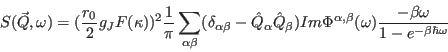
Summary: For the neutron scattering cross section we need the function $Im \chi^{\alpha\beta}(\omega+i\delta)/(1-\exp(-\beta\omega)$, where $\chi^{\alpha\beta}(z)$ is the frequency dependent part of the dynamic susceptibility $\chi^{\alpha\beta}(z)$ for spin components $J^\alpha$,$J^\beta$, which is related to the corresponding relaxation function $\Phi^{\alpha,\beta}$ by

$$\chi^{\alpha\beta}(z) = \chi^{\alpha\beta}(0) - \beta z \Phi^{\alpha\beta}(z)$$

For the full dynamical susceptibility we need the static suseptibility $\chi^{\alpha\beta}(0)$ which in lowest order in the exchange interaction is given by

$$\chi^{\alpha\beta}(0) = \sum_\nu (J^\alpha_\nu)^\dagger \beta P_\nu J^\beta_\nu$$

The above relaxation function is calculated with help of the Mori-Zwanzig projection formalism by

$$\Phi^{\alpha\beta}(z)=\sum_{\mu\nu} (J^\alpha_\nu)^*\Phi_{\nu\mu}(z)J^\beta_\mu$$

where $\nu$ denotes a transition from $n_1$ to $n_2$ between crystal field levels of the magnetic ion. The partial relaxation functions are obtained by solving the matrix equation

$$\Phi_{\nu\mu}(z)= [\Omega^{-1}]_{\nu\mu}P_\mu$$

with

$$\Omega_{\nu\mu}(z)= (z-\omega_\nu)\delta_{\nu\mu} -M_{\nu\mu}(z)/P_\mu$$

where $\omega_\nu =E_{n_2}- E_{n_1}$ is the energy difference of cf-levels.

Only terms in lowest order in the el-ion interaction are kept. We neglect frequency shifts due to the electron-ion interaction. Then the memory function is purely imaginary (with a negative sign).

Note that compared to our paper BFK, Z.Physik B28, 9-18, 1977 we have used here a different sign-convention.

For numerical reasons it is more convenient to calculate the relaxation function in the following way:

$$\Phi_{\nu\mu}(z)= P_\nu[\bar\Omega^{-1}]_{\nu\mu}P_\mu$$

with

$$\bar \Omega_{\nu\mu}(z)= P_\nu(z-\omega_\nu)\delta_{\nu\mu} - M_{\nu\mu}(z)$$

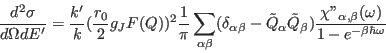
From the relaxation function we get for the dynamic scattering cross section

$${d^2\sigma \over d\Omega d E'} = {k' \over k}S(\vec Q,\omega)$$

with

$$S(\vec Q, \omega)=({r_0\over 2}g_J F(\kappa))^2{1\over \pi }... ...\beta}(\omega){-\beta \omega \over 1-e^{-\beta \hbar \omega}}$$

Here the scattering function depends only on the scattering vector $\vec Q = \vec k - \vec k'$ and the energy loss $(\hbar)\omega =E(k)-E(k')$ Note that in our formulas $\omega$ contains a factor $\hbar$ and is the energy loss. If we want to have meV as energy unit and Kelvin as temperature unit, we have to write $\beta= 11.6/T$.

For the analysis of polarised neutron scattering the different spin-components $S^{\alpha\beta}(\vec Q,\omega)$ of $S$ are needed. These are defined by

$$S(\vec Q,\omega)= \sum_{\alpha\beta}(\delta_{\alpha\beta} - \hat Q_\alpha \hat Q_\beta)S^{\alpha\beta}(\vec Q,\omega)$$

with

$$S^{\alpha\beta}(\vec Q,\omega)= Im \chi^{\alpha\beta}/(1-e^{... ...\beta}(\omega){-\beta \omega \over 1-e^{-\beta \hbar \omega}}$$

The complex dynamic susceptbility is calculated from

$$\chi^{\alpha\beta}(\omega)= \chi^{\alpha\beta}(0)-\beta \ome... ...ha_\mu)^*(P_{\mu\nu}-\omega \Phi_{\mu\nu}(\omega ))J^\beta_\nu$$

where the static susceptibilities $\beta P_{\mu\nu}$ are diagonal in our approximation.