Example - how to evaluate the crystal field of NdCu$_2$ using singleion

A simple input file is made up in the following:

• The first line in the input file sets the type of single ion module, for rare earth in spin-orbit coupling we use so1ion.
• Comment lines start with #.
• The type of ion has to be given plus several lines containing the crystal field parameters.

It follows an example, we take the values for NdCu$_2$ from literature [24]. Note that if the crystal field parameters are not known, there are different possibilities to obtain values, such as ab initio calculation, point charge calculations (use module pointc) and fitting to experimental data (see section 18).

#!MODULE=so1ion
#<!--mcphas.cf-->
# comment followed by
# the ion type and the crystal field parameters [meV]
 IONTYPE=Nd3+
 GJ=0.727273
# - note you can also do any pure spin problem by entering e.g. IONTYPE=S=2.5 
 B20=  0.116765                                           
 B22  =  0.134172                                           
 B40  =  0.0019225                                          
 B42  =  0.0008704                                          
 B44  =  0.0016916                                          
 B60  =  0.0000476                                          
 B62  =  0.0000116                                          
 B64  =  0.0000421                                          
 B66  =  0.0003662       
# instead of the Stevens parameters Blm 
# second order crystal field parameters Dx^2 Dy^2 and Dz^2 can be entered in meV
# - this corresponds to the Hamiltonian H=+Dx2 Jx^2+Dy2 Jy^2+Dz2 Jz^2
Dx2=0.1
Dy2=0
Dz2=0.4

1. The calculation of the single ion properties is performed using singleion with the option -r, i.e. type the command

   singleion -r Nd3p.sipf 20 0 0 0 0 0 0

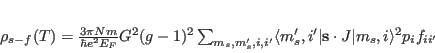
   Here Nd3p.sipf refers to the name of the single ion property file, the numbers 20 0 0 0 0 0 0 indicate the temperature in Kelvin, the 3 components of the applied magnetic field in Tesla and the 3 components of the exchange field in meV, respectively. Files Nd3p.sipf.levels.cef, Nd3p.sipf.trs and _Nd3p.sipf are generated in directory results, which must exist in order to run the program. _Nd3p.sipf contains the same information as the input file Nd3p.sipf, however it is not just copy, but formatted newly by the program singleion. In particular all numerical values are taken from the internal storage, thus this file can be used to check, whether the input file was read correctly (a typical error which can be detected this way would be to enter a number as ”4,25” instead of ”4.26” (correct way). In the first case a wrong number will be read and used in the calculation. The other output files of program singleion contain the results of the calculation, i.e. the diagonalisation of the Hamilton operator and the neutron scattering cross section. The program singleion outputs a variety of results, such as eigenvectors and energies of the crystal field states. In addition it provides the neutron powder cross section for each crystal field transition (in barn/sr) at a given temperature according to the formula

   
   

   $$\sigma(i\rightarrow k)=\left(\frac{\hbar \gamma e^2}{mc^2}\... ...a=x,y,z} \vert\langle i\vert J_{\alpha}\vert k\rangle\vert^2$$ (7)

   
   

   Note: in this calculation energy and Q dependence of the double differential scattering cross section are not considered and integration over all energies and scattering angles has been performed. In order to get a more realistic scattering intensity, the form factor (giving a $Q$ dependence), the factor $k'/k$ and the Debye Waller factor $exp(-W(Q))$ should be considered.

   Here comes the output file results/Nd3p.sipf.levels.cef:

    
   #
   #
   #!d=10 sipffile=Nd3p.sipf T= 20 K Hexta=0 T Hextb=0 T Hextc=0 T Hxc1=0 meV  Hxc2=0 meV  
                                          Hxc3=0 meV   Ia=0  Ib=-1.25627e-15  Ic=5.58172e-16 
   #! Eigenvalues = -5.85363 -5.85363 -2.94823 -2.94823 -0.86682 -0.86682  1.39302  
                                          1.39302  8.27566  8.27566 
   #Eigenvectors [as colunmns]
   #Real Part
   -0.022805 -0.042996 +0.025080 -0.000746 -0.000979 +0.009997 +0.242313 -0.000570 +0.968599 +0.000466 
   +0.786799 -0.417315 -0.009191 -0.309074 -0.119114 -0.011666 +0.000725 +0.308423 -0.000020 +0.041658 
   +0.174846 +0.329651 -0.305620 +0.009088 +0.070534 -0.720191 -0.469697 +0.001105 +0.151679 +0.000073 
   -0.203103 +0.107725 -0.008431 -0.283518 +0.671893 +0.065804 +0.001456 +0.618963 -0.000080 +0.166744 
   -0.052032 -0.098100 +0.853917 -0.025393 +0.007647 -0.078084 -0.492365 +0.001158 +0.096278 +0.000046 
   +0.098100 -0.052032 +0.025393 +0.853917 -0.078084 -0.007647 +0.001158 +0.492365 -0.000046 +0.096278 
   +0.107725 +0.203103 -0.283518 +0.008431 -0.065804 +0.671893 -0.618963 +0.001456 +0.166744 +0.000080 
   -0.329651 +0.174846 -0.009088 -0.305620 -0.720191 -0.070534 +0.001105 +0.469697 -0.000073 +0.151679 
   -0.417315 -0.786799 -0.309074 +0.009191 +0.011666 -0.119114 -0.308423 +0.000725 +0.041658 +0.000020 
   +0.042996 -0.022805 +0.000746 +0.025080 +0.009997 +0.000979 -0.000570 -0.242313 -0.000466 +0.968599 
   #Imaginary Part
   0         0         0         0         0         0         0         0         0         0         
   0         0         0         0         0         0         0         0         0         0         
   0         0         0         0         0         0         0         0         0         0         
   0         0         0         0         0         0         0         0         0         0         
   0         0         0         0         0         0         0         0         0         0         
   0         0         0         0         0         0         0         0         0         0         
   0         0         0         0         0         0         0         0         0         0         
   0         0         0         0         0         0         0         0         0         0         
   0         0         0         0         0         0         0         0         0         0         
   0         0         0         0         0         0         0         0         0         0
   

   Here comes the output file results/Nd3p.sipf.trs:

   #output file of program mcdisp version 5.2Sat Oct 31 04:57:16 2015
   #!<--mcphas.mcdisp.trs-->
   #*********************************************************************
   # mcdisp - program to calculate the dispersion of magnetic excitations
   # reference: M. Rotter et al. J. Appl. Phys. A74 (2002) 5751
   #            M. Rotter J. Comp. Mat. Sci. 38 (2006) 400
   #*********************************************************************
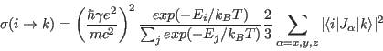
   #(*)The unpolarized powder average neutron cross section sigma for each transition 
   #   is calculated neglecting the formfactor, the Debye Wallerfactor, factor k'/k as follows:
   #-------------------------------------------------------------- 
   #            Transition intensities in barn/sr.                |
   #                                                              |
   # =                                                            |
   # |                           2                                |
   # |     = const wi  |<i|M |k>|                                 |
   # |                      T                                     |
   # =                                                            |
   #  E -> E                                                      |
   #   i    k                                                     |
   #                                                              |
   #                            with                              |
   #                                                              |
   #                      - E /T                                  |
   #                     e   i                                    |
   # wi    = const --------------                                 |
   #               ----    - E /T                                 |
   #               >    n e   i                                   |
   #               ----  i                                        |
   #                i                                             |
   #                                                              |
   #                                                              |
   #                                -----                         |
   #                      2     2   \                        2   |
   #        |<i,r|M |k,s>|   = ---   >     |<i,r|M -<M >|k,s>|    |
   #               T            3   /             u   u           |
   #                                -----                         |
   #                             u = x,y,z                        |
   #                                                              |
   #                                                              |
   #                             and                              |
   #                                                              |
   #                                   1       2                  |
   #                  const  =      ( --- r   )                   |
   #                                   2   0                      |
   #                                                              |
   #                                      -12                     |
   #                  r     = -0.53908* 10    cm                  |
   #                   0                                          |
   #                                                              |
   #                                                              |
   #                 M   =  L  + 2 S  = g  J                      |
   #                                     J                        |
   #                                                              |
   #--------------------------------------------------------------|
   #                                                              |
   #                       1.Sum rule :                           |
   #                                                              |
   #                                                              |
   #  ----  =       2                                             |
   #  >     |     =--- *g *g *const * J(J+1) *wi                  |
   #  ----  =       3    J  J                                     |
   #   k     E -> E                                               |
   #          i    k                                              |
   #                                                              |
   #--------------------------------------------------------------|
   #                                                              |
   #                       2. sum rule :                          |
   #                                                              |
   #                                                              |
   #            ----  =            2                              |
   #            >     |         = --- * const*g *g *J(J+1)        |
   #            ----  =            3           J  J               |
   #             k,i   E -> E                                     |
   #                    i    k                                    |
   #-------------------------------------------------------------- 
   #! ninit= 1e+08 (max number of initial states) -do not modify: needed to 
                         count transitions
   #! pinit= 0 (minimum population number of initial states)-do not modify: needed 
                         to count transitions
   #! maxE= 1e+10 meV(maximum value of transition energy)-do not modify: needed to 
                         count transitions
   #! T= 20 K Ha=0 Hb=0 Hc=0 T
   #*********************************************************************
   #i j k ionnr transnr energy |gamma_s| sigma_mag_dip[barn/sr](*)    wnn'|<n|I1-<I1>|n'>|^2 
                         wnn'|<n|I2-<I2>|n'>|^2 ... with wnn'=wn-wn' for n!=n'  and wnn=wn/k_B T 
   1 1 1  1     1        -1e-06   0.578897   0.0255675            0  0.450589  0.128308
   1 1 1  1     2             0    1.97195   0.0870932     0.931383  0.981677 0.0588932
   1 1 1  1     2             0    1.97195   0.0870932     0.931383  0.981677 0.0588932
   1 1 1  1     3        2.9054   0.732717    0.023043     0.605775  0.115041 0.0119001
   1 1 1  1     3       -2.9054   0.732717  0.00427206     0.605775  0.115041 0.0119001
   1 1 1  1     4        2.9054   0.506209   0.0159196     0.147164   0.35519 0.00385427
   1 1 1  1     4       -2.9054   0.506209  0.00295142     0.147164   0.35519 0.00385427
   1 1 1  1     5       4.98681   0.619651    0.016806    0.0312924  0.427228  0.161131
   1 1 1  1     5      -4.98681   0.619651  0.000931608    0.0312924  0.427228  0.161131
   

2. at the end of the file results/Nd3p.sipf.trs the neutron scattering cross section of the different transitions is given as a list of energy (column 6) vs intensity (column 8). However by default only 5 pairs of levels are considered. In order to consider all possible pairs of levels (in our case 55), you have to enter the option -nt 55, i.e. issue the command

   singleion -r Nd3p.sipf -nt 55 20 0 0 0 0 0 0

   In order to calculate a spectrum these results have to be convoluted with the resolution function of a neutron spectrometer. This can be done by the program convolute. For example, the commands

   gauss 0.5 0.05 -4 4 $>$ res.dat

   convolute 6 8 results/Nd3p.sipf.trs 1 2 res.dat $>$ results/Nd3p.sipf.cvt

   create a Gaussian resolution function (of 0.5 meV full width half maximum stored in stepsize 0.5 meV from -4 to 4 meV) and convolute the calculated neutron transition energies vs intensities in file results/Nd3p.sipf.trs with this Gaussian resolution function. The step size of the output spectrum is 0.05 meV. The output spectrum is contained in file results/Nd3p.sipf.cvt.

3. Use program display to view the spectrum:

   display 1 2 results/Nd3p.sipf.cvt

   In order to create an image file for printing the viewed spectrum can be saved by either a printscreen or by using the option -o file.jpg of the display program. Such a jpg image is shown in figure 5.

   Figure 5: Calculated crystal field neutron spectrum of NdCu$_2$ at a temperature of 10 K. Horizontal axis is energy transfer in meV and vertical axis is neutron intensity in barns per meV and Nd atom and sr. [plot created by program display]

   
4. In order to calculate the magnetisation for our problem (in the paramagnetic state), the magnetic field has to be given in the command line and program singleion has to be started with the option -M, i.e.

   singleion -M -r Nd3p.sipf 10 0 0 1 0 0 0

   The numbers denote a temperature (10 K) and a field 1 Tesla along the z-axis. By default the results are written directly to the screen, however they can be piped into a file by

   singleion -M -r Nd3p.sipf 10 0 0 1 0 0 0 $>>$ results/moment.rtplot

   Here the ”$>>$” sign appends the ouput of each command, thus iterating the command for several different magnetic fields allows to calculate a magnetisation curve - fig. 6 shows the result.

   Figure 6: Calculated magnetic moment for field applied along $x$ direction ($c$ axis, note the notation of the crystal field $xyz$ axes with respect to the crystal lattice is $xyz\vert\vert cab$ in our example) of NdCu$_2$ at a temperature of 10 K. [plot created by program gnuplot]

   

5. In a similar way the temperature dependence of the susceptibility can be calculated, actually one calculates the magnetisation at variable temperature.

6. The crystal field contribution to the specific heat may be calculated from the output file results/Nd3p.sipf.levels.cf using the program cpsingleion, e.g.

   cpsingleion 10 100 1 results/Nd3p.sipf.levels.cef calculates the specific heat in the temperature interval 10-100 K with a step width of 1 K. Alternatively a comparison to experimental data can be made by cpsingleion 1 2 cpexp.dat results/Nd3p.sipf.levels.cef, where the temperatures are given in column 1 and the experimental specific heat in column 2 of file cpexp.dat. The calculated specific heat is compared to the experimental data and a standard deviation sta is calculated and output is written to stdout. Other quantities can be calculated using the options: -s (calculate entropy (J/molK) instead of cp), -f (calculate free energy (J/mol) instead of cp),-u (calculate magnetic energy (J/mol) instead of cp), -z (calculate partition sum instead of cp). Fig. 7 shows an example.

   Figure 7: Calculated specific heat of NdCu$_2$ in zero magnetic field as calculated by cpsingleion (crystal field contribution) in comparison with experimental data [24]. The dashed line shows the results of a calculation, which in addition to the crystal field takes into account the two ion interaction in mcphas - see below and chapter 7. [plot created by program gnuplot]

   

7. The spin-disorder resistivity due to scattering of conduction $s$-electrons with the localised $f$-electrons via the exchange interaction can be calculated in the first Born approximation as [26],

   
   

   $$\rho_{s-f}(T) = \frac{3\pi N m}{\hbar e^2 E_F} G^2(g-1)^2 ... ... \vert {\mathbf s \cdot J} \vert m_s, i \rangle^2 p_i f_{ii'}$$ (8)

   
   

   where $G$ is the exchange constant, $p_i$ is the Bose factor $e^{-\beta E_i}/Z$ and $f_{ii'}$ is the Fermi function $2/(1+e^{-\beta(E_i-E_{i'})})$. The program rhoso1ion can be used to calculate this resistivity for magnetic ions in a crystal field. The wavefunctions $\vert i\rangle$ are taken from the file results/Nd3p.sipf.levels.cef output by singleion. The matrix elements of ${\mathbf s \cdot J}$ are calculated according to the formulae of Dekker [27]. rhoso1ion calculates only the sum in the above equation, however. The constant coefficient $\rho_0=(3\pi N m/\hbar e^2 E_F) G^2(g-1)^2$ is set to unity, or may be specified using the option -rho0 or -r. The syntax is otherwise the same as cpsingleion. For example, to calculate the resistivity from 10 to 100 K in 1 K steps with $\rho_0 = 0.2$ $\Omega$.cm, the command

   rhoso1ion 10 100 1 -r 0.2 -i results/Nd3p.sipf.levels.cef

   can be used. Alternatively, for comparison with data,

   rhoso1ion 1 2 rhoexp.dat -r 0.2 -i results/Nd3p.sipf.levels.cef

   can be used. Note that as the temperature dependence of the resistivity in this case is mainly a function of the Bose and Fermi functions, at high temperatures where all $2J+1$ crystal field levels are thermally occupied, the resistivity will saturate to a value $\rho_0 J(J+1)$.

Exercises:

• Use singleion to calculate the energies, eigenvectors and transition matrix elements (for inelastic neutron scattering) for Nd$^{3+}$ in an orthorhombic crystal field. Use the parameters given in section 6.3.