mcphas.ini - controlling the algorithm

Initial file containing algorithm control parameters, for instance the range and spacing of propagation vectors Q or the number of Monte Carlo trials for initial spin configurations - mind: this file is rewritten and reread when running the program and may be changed by the user in order to manipulate the running simulation.

mcphas.ini consists of several sections:

MCPHASE RUNTIME CONTROL:

this section contains the parameters controlling the status of the calculation.

XY PHASEDIAGRAM PARAMETERS:

here the temperature and field range and step widths of the calculation are specified. The definition of the x and y axis in terms of temperature and magnetic field is followed by the corresponding range and step width. An offset may be given for all field and temperature values. Note that for most cases of interest this offset is zero (T0=0, Ha0=0, Hb0=0, Hc0=0). For the simple case of calculating a Temperature-Field phase diagram It is just necessary to set xT=1 and give the temperature range by xmin/xmax/xstep. For field in b direction then just set yHb=1 and define the range in ymin/ymax/ystep. In case of non-orthogonal axes the applied magnetic field components $Ha, Hb, Hc$ refer to the orthogonal coordinate system defined with respect to the nonorthogonal lattice $\mathbf a,\mathbf b,\mathbf c$ as $Hb\vert\vert\mathbf b$, $Hc\vert\vert(\mathbf a \times \mathbf b)$ and $Ha$ perpendicular to $Hb$ and $Hc$.

GENERATION OF SPINCONFIGURATIONS:

at the beginning of the program some initial values of spin configurations are generated from a set of propagation vectors. This section defines the range of propagation vectors and the step width. Depending on the value of the propagation Q with respect to the primitive reciprocal lattice 1-, 2- or 3-dimensional simulations of magnetic lattices are possible. It is advisable to think carefully about the chosen range and spacing of Q vectors in order to limit calculation time.

For example a good starting point is to begin with a calculation with large step widths (e.g. 0.1) covering the Brillouin zone. This should give an idea of the propagation vectors which are stabilised. An advanced calculation could then fine tune the propagation and determine its accurate value (using small step widths in a limited area of the zone). The verbose option of mcphas allows to inspect the propagation vectors which are actually used in the calculation. Trick: in order to get a quick overview of the q-vector range covered by the mcphas simulation start mcphas, exit and just type felog ./results/mcphas.qvc (need perl,perldl,pdl,pgplot packages).

In order to limit calculation time, the maximum periodicity of the magnetic unit cell with respect to the crystallographic unit cell (maxqperiod) and the maximum number of spins in the magnetic unit cell (maxnofspins) can be limited. Also the maximum number of test spin configurations in the internal table can be limited (maxnoftestspincf). A critical feature with respect to calculation time is also the number of spin configurations which are generated by a random process from a tabulated SPINCONFIGURATIONS during the calculation.

In summary the variables in this section are mainly important to adapt the program to a given computer system with finite speed. They have to be set to optimise between speed and accuracy of the calculation. In order to find appropriate values it is best to perform some calculations and restrict the parameters step by step if insufficient speed is obtained. Also the examples included in the program package may serve as starting points.

PARAMETERS FOR SUB FECALC SELFCONSISTENCY PROCESS:

the most important procedure in the module mcphas is the sub fecalc. In this part of the program the self consistent calculation of the magnetic moment configuration is performed as shown schematically in fig. 8. In the mean field approximation the Hamiltonian (1) is approximated by a sum over the $N_b$ sites in the magnetic supercell

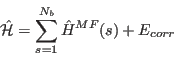$${\hat \mathcal H}=\sum_{s=1}^{N_b} \hat H^{MF}(s) + E_{corr}$$ (13)

with the single ion Hamiltonian

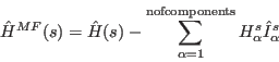$$\hat H^{MF}(s)= \hat H(s) - \sum_{\alpha=1}^{\rm nofcomponents} H_{\alpha}^s \hat I_{\alpha}^s$$ (14)

In case of module so1ion in it's simplest application with ${\rm nofcomponents}=3$ interaction operators only, the interaction operators are defined to be equal to the total angular momentum, i.e. $\hat I_{\alpha}=\hat J_{\alpha}$ (with the magnetic moment $\mathbf M=g_{J} \mu_B \langle \hat \mathbf J \rangle$ ) and the single ion Hamiltonian is given by

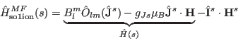$$\hat H^{MF}_{\rm so1ion}(s)= \underbrace{ B_l^m \hat O_{lm}... ...bf H} }_{\hat H(s) }- {\hat \mathbf I}^s \cdot {\mathbf H}^s$$ (15)

Note, here ${\mathbf H}^s$ denotes the exchange field at the site $s$ and ${\mathbf H}$ denotes the applied magnetic field.

The correction term is defined by

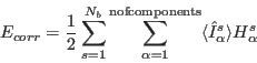$$E_{corr}=\frac{1}{2}\sum_{s=1}^{N_b}\sum_{\alpha=1}^{\rm no... ...onents} \langle {\hat I}^s_{\alpha} \rangle {H}^s_{\alpha}$$ (16)

and the components exchange fields ${\mathbf H}^s$ are given by

$$H^s_{\alpha}=\sum_{\mathbf G'}\sum_{s'=1}^{N_b}\sum_{\beta... ...athbf G'+\mathbf r_{s'})) \langle \hat I^{s'}_{\beta} \rangle$$ (17)

The exchange fields ${\mathbf H}^s$ and the moments $\langle {\hat\mathbf I}^s \rangle$ are determined in a self consistent way. For a given magnetic unit cell and initial configuration of moments the exchange fields are calculated according to equation (17). Then, for each magnetic ion the single ion property module is taken and the moment $\langle {\hat\mathbf I}^s \rangle$ is calculated from it's mean field. The mean fields are used again in equation (17) and so on .... until convergence is reached. Then, the free energy per site $f$

$$f = -kT\frac{1}{N_b}\sum_s \ln(z_s) + \frac{E_{corr}}{N_B}$$ (18)

$$z_s = \sum_i \exp(-\epsilon^s_i/kT) \, {\rm\dots partition \, sum \, of \, the \, site} \, s$$ (19)

$$\epsilon_i^s \, {\rm\dots \, eigenvalues \, of \, }\hat H^{MF}(s)$$

of the stabilised configuration is calculated (this is why this sub is called fecalc). The free energies of a lot of different stabilised configurations have to be compared in order to find out which configuration has lowest free energy, i.e. is stable in thermal equilibrium.

It may happen that this process does not converge due to bad choice of the initial configuration, therefore a maximum number of mean field loops has to be given by the user. The results of a calculation may be significantly influenced by changing parameters such as the maximum number of iteration loops in this section. In fact the simulation is always a compromise of calculation time and accuracy: if only a few initial spin configurations are tried at each (H-T) point, the calculation speed is fast, however it is possible that the program misses the magnetic structure with the lowest free energy. The same holds if other critical parameters of the simulation are restricted too much.

OUTPUT OF PHYSICAL PROPERTIES:

Some options for the output of the calculation can be changed in this section.

Figure 8: Mean field process of sub fecalc.